We'll need to determine the ratio spread (highest
ratio and lowest ratio).
1. Determination of the "highest ratio"
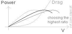
Usually the "highest ratio" is selected so that it will allow the
achievement of the
maximum possible speed. Nevertheless, an higher ratio is also used
to benefit highway fuel economy. (But it would not achieve the top speed.)
Thus, we need to know the vehicle's maximum speed, using the given power.
|
 |
1.1. Available power?
Considering that the engine power is Pe =
[hp],
and the transmission efficiency (incl. rolling resistance) is Eff =
[%],
and the available power (Pt) of the transmission will be:
Pt = Pe × Eff
[hp] =
[w].
1.2. Thrust force?
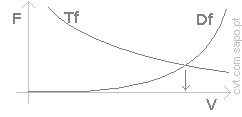
At a speed v (m/s), the Thrust_force will be Tf = Pt/v
= /v [N]
|
 |
1.3. Drag force?
To determine the maximum speed we must also calculate the Drag_force,
Df.
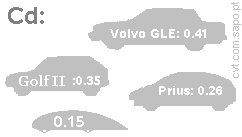
The Df = Cd × ½ × r × v² × A
where:
Cd: drag force coefficient:
r: air density (=1.2 [kg/m³])
v: vehicle velocity (m/s) |
 |
| A : -Vehicle's projected
frontal area: [m²]
|
 |
1.4. Maximum speed?
Therefore the maximum velocity will be calculated by equating the
Thrust_force to the Drag_force (Tf = Df), and solving for
the velocity:
v³ = Pt / (Cd × ½ × r × A) thus
v.max
[m/s] (=[km/h]
=[mph]); |
 |
1.5. Highest ratio?
Considering that the maximum power is at
rpm (rpm.P),
the wheel diameter is [inch]
(w.diam, use the calculator at the right → ),
and the differential ratio is
:1 ,
the highest ratio (high.ratio) will be calculated by the equation:
v.max = (rpm.P ×2×3.1416/60) × ((w.diam×0.0254)/2) /
(high.ratio×differential)
thus
high.ratio = (rpm.P ×2×3.1416/60) × ((w.diam×0.0254)/2)
/ (v.max×differential)
and therefore the high.ratio
Note: this “highest ratio” value was selected in order to optimize the
maximum speed. |

|
Tire
width
[mm]:
|
Aspect
ratio:
|
Wheel
size
[inch]
|
|
2. Determination of the lowest ratio
2.1. Force due to the slope?
Consider that the car must be able to start moving uphill, fully loaded.
The vehicle's mass is
[kg] and the maximum
load is [kg] (incl.
passengers).
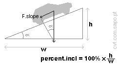
The slope inclination, (percent.incl), is
[%] and the safety
factor is .
The force due to the slope will be:
F.slope = (mass+load) × 9.81 × (percent.incl/100) ×
safety / Eff
[N];
(note: Eff is the transmission efficiency ). |
 |
2.2. Available tangential force in the tyres:
The maximum engine torque is
[Nm] .
However when starting to move the clutch slip results in an efficiency of
% (clutch.eff).
So the tangential force in the tyres will be:
F.tyres = torque × clutch.eff × low.ratio ×
differential / ((w.diam×0.0254)/2) |
 |
2.3. lowest ratio?
Equating F.slope = F.tyres and isolating low.ratio
results:
low.ratio = F.slope × ((w.diam×0.0254)/2) / (torque×clutch.eff×differential)
thus
low.ratio
:1
So, at this point we already know the required “lowest ratio” and “highest
ratio”. |
 |
3. Addition of an external fixed ratio to obtain
symmetric ratios:
The previous calculations
resulted in: low.ratio:
high.ratio :.
However a V-Belt CVT usually generates (almost*)
symmetric extreme ratios:
[ low.ratio × cf = 1 /
high.ratio ]
because both pulleys move
apart by equal amounts (alternatively).
*Note: cf =
is a correction factor. Lower
cf values are used to lower the
whole ratio span within the CVT (cf = 0.91 .. 0.99) which is
beneficial.
Therefore, we must add a fixed reduction
after the V-Belt CVT.
This way the V-Belt CVT will be able to have a (almost)
symmetric ratio span.
The fixed reduction ensures that
the final ratio span will be exactly
from
low.ratio to
high.ratio.
Therefore, we must add (in series)
a final (fixed) reduction with a
ratio of :
k = SquareRootOf ( low.ratio×high.ratio ×cf ), thus
k
.
Now we must calculate the new CVT's
high and low ratios. These will result from
dividing each of initial
low.ratio and high.ratio by
k.
Conclusion:
in this case the CVT's symmetric ratios will be
=s.l.ratio, and
=s.h.ratio. |
 |
4. CVT dimensions:
4.1. Pulley:
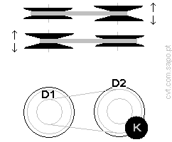
Considering that the smaller diameter (D1) is
[mm]
and that the bigger is (D2) will be so that D1/D2=s.h.ratio.
Thus D2 = D1/s.h.ratio
[mm]. |
 |
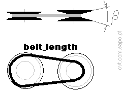
Specify the pulley groove angle: betha =
deg.
4.2. Belt:
Knowing that the pulleys centre-to-centre distance is a=[mm]
(note: it must be greater than
[mm]),
...the belt_length will be 2×a+(PI/2)×(D2+D1)+(D2-D1)×(D2-D1)/(4×a).
Thus the belt_length
[mm].
|
 |
5. Velocities:
(considering the maximum power regime)
5.1. Velocities in the lowest ratio:
Rotational speed driver pulley =
[rpm]; (n1);
Rotational speed driven pulley
[rpm]; (n2=n1/s.l.ratio);
Belt_speed = [m/s];
((n1×2×PI/60)×(D1/2))
|

|
5.2. Velocities in the highest ratio:
Rotational speed driver pulley =
[rpm]; (n1);
Rotational speed driven pulley
[rpm]; (n2=n1/s.h.ratio;);
Belt_speed = [m/s];
|
 |
6. Forces:
6.1. Friction coefficient:
Consider the coefficient of friction is mu=.
Therefore, the effective friction coefficient will be calculated by
mu.e = mu/sin(betha/2)
.
|
|
6.2. Belt tensions in the lowest ratio:
The lowest ratio is .
In the following, we will use D1=[mm]
for the driver pulley,
and D2=[mm] for
the driven pulley. |
 |
The smallest belt wrap angle is calculated by
2×acos((D2-D1)/(2×a)), thus alpha
[deg]; |
 |
(Note: the following is
not valid for pushbelt CVTs)
The ratio of the belt forces will be exp(mu.e×alpha),
so T12 = ;
Belt tension load T1 will be (Pe/Belt_speed)/(1-1/T12)
= [N];
(Note:Pe is the engine power).
Belt tension load T2 will be T1/T12 =
[N]; |
 |
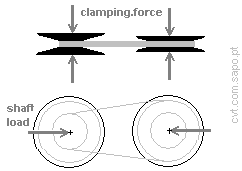
And the shaft load can be calculated by:
(shaft.load)² = T1×T1+T2×T2-2×T1×T2×cos(alpha);
Thus, shaft.load = [N];
Axial clamping.force = ( Pe/Belt_speed )/ mu.e
= [N]
|
 |
6.3. Belt tensions in the highest ratio:
The highest ratio is .
Now the driver pulley is D1=[mm],
and the driven pulley is D2=[mm].
|
 |
| The smallest belt wrap angle is alpha
[deg]; |
 |
(Note: the following is
not valid for pushbelt CVTs)
The ratio of the belt forces will be T12 =
;
Belt tension load T1:
[N];
Belt tension load T2 =
[N]; |
 |
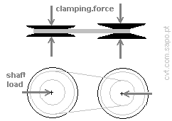
And the shaft.load =
[N];
Axial clamping.force = ( Pe/Belt_speed )/ mu.e
= [N].
|
 |